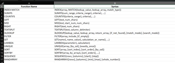
Advanced Excel Functions for Data Analysis
Do you use Excel every day but feel like you’re missing its full potential?
Table of Contents
In this post, we’ll break down the most advanced Excel functions for data analysis, explain when and how to use them, and show you practical examples that will change the way you work with data.
🔍 Why Use Advanced Excel Functions?
1. 🕒 Save Time on Repetitive Tasks
Advanced functions like SUMIFS, INDEX-MATCH, FILTER, and XLOOKUP allow you to:
- Automate calculations
- Avoid manual lookups
- Summarize large datasets in seconds
👉 Example: Instead of filtering and manually summing values, a single SUMIFS formula can return monthly sales by product or region instantly.
2. 🧠 Reduce Human Error
Manual copy-paste and filtering often lead to mistakes. Advanced formulas help:
- Standardize logic
- Minimize manual interventions
- Automatically update results when data changes
📌 Pro tip: Use IFERROR or ISNUMBER to clean up messy results or missing data automatically.
3. 📊 Dynamic Reporting and Dashboards
With functions like OFFSET, INDIRECT, FILTER, and LET, you can:
- Build interactive dashboards
- Link dropdowns to charts
- Make reports that update with just a change in input
🛠 Tip: Pair with Form Controls (slicers, dropdowns) to build user-friendly, no-code dashboards.
4. 🔄 Easier Data Cleaning & Transformation
Functions like TEXTSPLIT, TEXTAFTER, TRIM, SUBSTITUTE, and UNIQUE help you:
- Clean raw data faster
- Split or reformat columns
- Remove duplicates
These are must-haves when working with messy exports from CRMs, ERPs, or databases.
5. 🔁 Enable Scalable Templates
Using dynamic functions like LAMBDA, SEQUENCE, and LET, you can:
- Create reusable templates
- Abstract complex logic into custom mini-functions
- Scale from 100 to 100,000 rows easily
📦 Example: Build a monthly sales template where only the data changes — not the logic.
6. 🧩 Automate Decision Logic
Functions like IFS, CHOOSE, and SWITCH help automate:
- Grading systems
- Risk evaluations
- Financial triggers and alerts
You set the logic once, and Excel handles the decisions every time data updates.
🔍 INDEX-MATCH: A Better Alternative to VLOOKUP
If you’ve been using VLOOKUP for years, it’s time to upgrade! The INDEX-MATCH combo is more powerful, flexible, and reliable. Here’s why smart analysts and Excel pros prefer it:
✅ Why INDEX-MATCH is Better than VLOOKUP:
- Lookup Left or Right: VLOOKUP can only search to the right. INDEX-MATCH can lookup in any direction — even to the left!
- Faster with Big Data: INDEX-MATCH is more efficient with large data sets and won’t slow down as much as VLOOKUP.
- No Column Breaks: VLOOKUP uses column numbers, which break if columns are added/removed. INDEX-MATCH uses named columns or ranges — no breakage!
- More Accurate: INDEX-MATCH allows exact or closest match, with more control over the logic.
📘 Basic Syntax:
=INDEX(array, MATCH(lookup_value,lookup_array,match_type))
🧪 Simple Example:
Suppose you have a table like this:
Name     | Sales
-------- | ------
Alice    | 1500
Bob      | 1200
Charlie  | 1700
To find the sales of “Bob”:
=INDEX(B2:B4, MATCH("Bob", A2:A4, 0))
This formula looks for “Bob” in column A and returns the matching value from column B. It’s accurate, flexible, and works even if you rearrange the columns.
📌 Pro Tip:
Combine with IFERROR to avoid ugly #N/A errors:
=IFERROR(INDEX(B2:B4, MATCH("Bob", A2:A4, 0)), "Not Found")
Bottom line: Once you master INDEX-MATCH, you’ll rarely go back to VLOOKUP. It’s the foundation of smart, scalable Excel models.
🔎 VLOOKUP: The Classic Lookup Tool
VLOOKUP (Vertical Lookup) is one of the most widely used functions in Excel. It helps you search for a value in the first column of a table and return a corresponding value from another column.
📘 Basic Syntax:
=VLOOKUP(lookup_value, table_array, col_index_num, [range_lookup])
🧪 Simple Example:
Suppose you have this table:
Name     | Sales
-------- | ------
Alice    | 1500
Bob      | 1200
Charlie  | 1700
To find the sales for “Bob”, you can use:
=VLOOKUP("Bob", A2:B4, 2, FALSE)
This tells Excel to:
- Look for “Bob” in column A (the first column of the range)
- Return the value from column 2 (Sales)
FALSEensures an exact match
⚠️ Common Limitations:
- 🔁 Only searches to the right — can’t return values from columns to the left of your lookup column
- 📉 Breaks if you add/remove columns — because it uses a fixed column number
- 🚫 Slower with large data — especially when used many times in a workbook
Still, VLOOKUP is great for beginners and quick lookups in simple datasets. But if you want flexibility and scalability, consider switching to INDEX-MATCH.
🔎 XLOOKUP – The Modern Replacement for VLOOKUP and HLOOKUP
💡 What is XLOOKUP?
XLOOKUP is a powerful Excel function introduced as a modern alternative to the older VLOOKUP and HLOOKUP. It allows you to look up a value in a range or array and return a corresponding value from another range — both vertically and horizontally.
Syntax:
=XLOOKUP(lookup_value, lookup_array, return_array, [if_not_found], [match_mode], [search_mode])
⚙️ Key Differences from VLOOKUP
| Feature | XLOOKUP | VLOOKUP |
|---|---|---|
| Search direction | Vertical or horizontal | Vertical only |
| Column position | Any direction (left or right) | Only right of the lookup column |
| Error handling | Built-in if_not_found | Use IFERROR separately |
| Dynamic arrays | Yes | No |
| Approximate match | Custom match modes | Limited (TRUE/FALSE) |
📊 Real-World Use Cases
- 🔁 Replacing old
VLOOKUPorINDEX-MATCHformulas - 📋 Looking up customer names from IDs in CRMs
- 📦 Returning product price, availability, or region from a master list
- 📆 Time-based lookups: match the closest date in financial models
🧪 Example
Suppose you have a table:
Product   | Price
--------- | -----
Apple     | 100
Banana    | 60
Orange    | 80
Formula:
=XLOOKUP("Banana", A2:A4, B2:B4)
Result: 60
Pro tip: Combine with TEXTSPLIT, FILTER, or LET for even more automation.
📈 SUMIFS & COUNTIFS: Powerful Multi-Criteria Tools
When you need to sum or count values based on multiple conditions, SUMIFS and COUNTIFS are your best friends. They’re essential for analyzing large datasets quickly and accurately.
🔢 What They Do:
- SUMIFS: Adds numbers that meet one or more criteria
- COUNTIFS: Counts cells that meet one or more criteria
🧪 Example Dataset:
Region   | Product | Sales
-------- | ------- | -----
West     | Apple   | 150
East     | Banana  | 200
West     | Apple   | 180
East     | Apple   | 170
🧮 Example 1: SUMIFS
Goal: Get total Apple sales in the West region
=SUMIFS(C2:C5, A2:A5, "West", B2:B5, "Apple")
This will return 330 (150 + 180).
🔢 Example 2: COUNTIFS
Goal: Count how many times Apple was sold in the East region
=COUNTIFS(A2:A5, "East", B2:B5, "Apple")
This will return 1.
⚡ Why It Matters:
- 📊 Real-time analysis: Formulas update when data changes
- 📉 No manual filters: Avoid error-prone filtering and copying
- 📁 Cleaner reports: Use within dashboards, pivots, or summary tables
Pro tip: You can also use SUMIFS and COUNTIFS with date ranges, dropdown selections, or wildcard characters (*).
🔤 Mastering TEXT Functions: LEFT, MID, RIGHT, TEXTSPLIT
TEXT functions help you clean and extract useful parts of strings — especially helpful when dealing with unstructured data from CRMs, ERPs, or exported reports.
✂️ 1. LEFT
Use: Extracts characters from the beginning of a string.
=LEFT("Invoice12345", 7)
Result: Invoice
🔍 2. MID
Use: Extracts characters from the middle of a string, based on start position and length.
=MID("Product-5678", 9, 4)
Result: 5678
🏁 3. RIGHT
Use: Extracts characters from the end of a string.
=RIGHT("Customer_ABC", 3)
Result: ABC
🔗 4. TEXTSPLIT
Use: Splits text into multiple columns or rows based on a delimiter (Excel 365+).
=TEXTSPLIT("Name:Email:Phone", ":")
Result: {Name, Email, Phone}
🧹 Real-World Uses:
- 📄 Extract order numbers, customer IDs, or codes from longer strings
- 📦 Clean SKU formats or separate parts of product descriptions
- 📧 Parse emails or combined fields into structured columns
Pro tip: Combine with TRIM, SUBSTITUTE, or TEXTAFTER for more powerful cleanup operations.
🧲 FILTER – Extracting Data with Conditions
🔍 What Does the FILTER Function Do?
The FILTER function returns a dynamic array of values that meet one or more specified conditions. It’s a game-changer for building live, auto-updating reports without using manual filters, pivot tables, or helper columns.
🧪 Syntax Explained
=FILTER(array, include, [if_empty])
- array: The range to return from
- include: The condition(s) to apply
- if_empty: Optional value if no match is found
📋 Example:
Filter products with sales over 1000:
=FILTER(A2:B10, B2:B10 > 1000, "No results")
🚀 Why FILTER Beats Manual Filtering
- 🔄 Auto-updates: Changes dynamically when the source data changes
- 📤 No export needed: Useful in shared workbooks or dashboards
- 🧱 Build blocks: Combine with
SORT,UNIQUE, orLETfor live views - 🎯 Multi-condition support: Can use AND/OR logic for complex filters
📊 Use Cases:
- ⏱ See only pending tasks by status or owner
- 📈 Show sales for a selected region or date range
- 👥 Filter customers with overdue balances
Pro tip: Nest FILTER inside IF or CHOOSECOLS to build interactive dashboards without VBA or scripts.
🧠 LET & LAMBDA – Custom Functions and Performance Boost
LET Function: Improve Readability & Performance
The LET function allows you to assign names to calculation results. It makes formulas easier to read and faster to run.
=LET(x, A1*2, y, A2*3, x + y)What it does: Calculates x as A1*2, y as A2*3, then returns x + y.
- ✅ Reduces repetitive calculations
- ✅ Makes formulas easier to debug
LAMBDA Function: Create Your Own Functions
The LAMBDA function lets you define your own custom Excel functions without using VBA.
=LAMBDA(x, x^2)This returns a formula that squares any input x. Pair it with LET or Named Ranges to reuse it like a built-in function.
Real-Life Use Case:
Need to calculate weighted scores repeatedly? Define a LAMBDA function once and reuse it with different inputs.
=LAMBDA(score, weight, score * weight / 100)(85, 40)
Result: 34 — no need to write new logic each time!
💡 Combine LET and LAMBDA for clean, dynamic, and efficient Excel models—great for automation and reporting.
🔗 Dynamic Arrays – The Backbone of Modern Excel
What Are Dynamic Arrays?
Dynamic Arrays automatically spill values into adjacent cells based on a single formula. No more copying formulas or using helper columns! This revolutionizes how we analyze and report data.
💡 Key Functions That Use Dynamic Arrays
FILTER– Returns values based on conditionsUNIQUE– Extracts distinct values from a rangeSORT– Sorts values alphabetically or numericallySORTBY– Sorts based on another range or conditionSEQUENCE– Generates lists of numbersRANDARRAY– Creates random arrays
⚙️ How It Works
When you enter a formula like:
=UNIQUE(A2:A100)It automatically “spills” the unique values into the cells below, adjusting dynamically as the data changes.
🧩 Real-Life Use Cases
- 📋 Auto-generating dropdown lists using
UNIQUE - 📊 Live sales reports filtered by region using
FILTER - 📅 Creating a list of dates using
SEQUENCE
🚫 No More:
- Dragging formulas down rows
- Manually updating helper columns
- Broken formulas from missing ranges
Pro Tip: Use the # symbol (e.g., <code=A1#) to refer to the entire spilled array for further calculations.
✅ Dynamic Arrays are the foundation of Excel’s modern formula engine—combine them with LET, LAMBDA, and XLOOKUP to build truly automated spreadsheets.
You don’t need to be a data scientist to analyze data like one. By mastering these advanced Excel functions, you can make better decisions, save time, and stand out professionally.


